Do I Call or Fold? How Bayes’ Theorem Can Help Navigate Poker’s Uncertainty, Part 1

Let’s start out with a one-question quiz, to see how sharp you are. Its application to poker will become clear later.
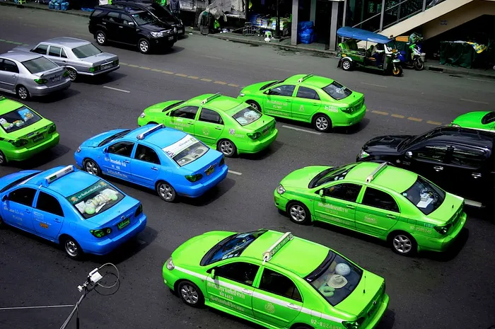
A cab was involved in a hit-and-run accident at night. Two cab companies, the Green and the Blue, operate in the city. You are given the following data:
- 85% of the cabs in the city are Green and 15% are Blue.
- A witness identified the cab as Blue.
- The court tested the reliability of the witness under the same circumstances that existed on the night of the accident and concluded that the witness correctly identified each one of the two colors 80% of the time and failed 20% of the time.
What is the probability that the cab involved in the accident was Blue? Take a minute to come up with your answer before reading on.
Ready?
In this two-part article, I’m going to introduce you to a mathematical concept called Bayes’ Theorem. In short, it’s a way of using imperfect information to improve our estimate of an unknown probability.
As you know, this is a task that comes up constantly in poker. For example, what is the probability that the guy in Seat 4 is bluffing — and how does our estimate of that probability change when we notice a tell on him? Bayes’ theorem tells us how to arrive at the most accurate answer.
However, becoming sufficiently familiar with the theorem to apply it takes some time and effort. If you’re interested in adding this tool to your mental toolbox, stick with me while I walk you through a couple of non-poker examples. Then next week in the second part I’ll show how the same principles apply in poker.
Was the Cab Blue or Green? Integrating Witness Reliability and Prior Probability
The taxicab problem is a famous one in the world of experimental psychology. It’s found in perhaps the most important book ever written on the flawed ways that people make decisions, Judgment Under Uncertainty: Heuristics and Biases by Daniel Kahneman, Paul Slovic, and Amos Tversky.
“A large number of subjects have been presented with slightly different versions of this problem, with very consistent results,” write the authors. “The [most common] answer is .80, a value which coincides with the credibility of the witness and is apparently unaffected by the relative frequency of Blue and Green cabs.”
So if your answer was 80%, you’re typical — but wrong. If you’re like most people, you had difficulty integrating two separate pieces of information: the witness’s reliability and the relative numbers of Blue and Green cabs.
Let’s work through the real answer. To simplify things, and to let us use whole numbers instead of percentages, let’s assume that the city has exactly 100 cabs, meaning 85 of them are Green company cabs and 15 of them are Blue company cabs.
If a cab is Blue, this witness will correctly identify it as Blue 80% of the time, and wrongly identify it as Green 20% of the time. Similarly, if a cab is Green, she will correctly identify it as Green 80% of the time, and wrongly identify it as Blue 20% of the time.
We can use this information to construct a small table:
| Green cab | Blue cab | Totals | |
|---|---|---|---|
| Witness says Green | 68 | 3 | 71 |
| Witness says Blue | 17 | 12 | 29 |
| TOTALS | 85 | 15 | 100 |
When the cab is Green, the witness correctly identifies it as Green 80% of the time. With 85 Green cabs, that’s 68 identifications of Green cabs as Green, and 17 identifications of Green cabs as Blue — her erroneous 20%. That’s the first column of numbers in the table.
Similarly, she identifies the Blue cabs correctly 12 times, and wrongly calls them Green 3 times — the same 80% and 20%. Those go into our second column.
If we were to parade all 100 cabs before this witness, then, she would call out “Green” 71 times, and “Blue” 29 times, as shown in the “Totals” column.
The critical question is this: When the witness says that a cab is Blue, what is the probability that it actually is Blue? We get the answer from the second line of numbers in our table. Of the 29 identifications she makes of Blue cabs, only 12 are actually Blue, while 17 are actually Green.
The final answer, then, is that when the witness says that the cab was Blue, the probability of the cab actually being Blue is only 12 out of 29, or about 41%. Because there are only two possible cab colors, we immediately also know that the probability of the cab actually being Green is 100% minus 41%, or 59%.
Think about the implications. Even though this witness is 80% accurate, when she identifies a cab as having been Blue, it is still more likely that the cab was actually Green! This is the part of the problem that people find difficult to grasp.
The correct answer relies heavily on the fact that there are a whole lot more Green cabs than Blue. It might help to consider other cities, with different numbers of Blue and Green cabs.
If this incident had happened in a city with 99 Green cabs and 1 Blue, you can probably intuit that, even when the witness says “Blue,” she’s almost certainly wrong, just because Blue cabs are so rare. Conversely, if this happened in a city with 1 Green cab and 99 Blue, and the witness said, “Blue,” she’s virtually certain to be correct.
In both cases, we are 99% confident of the correct color of the cab even before the witness speaks, so unless she is absolutely perfect in her identification, that fact will weigh much more heavily than her word. Her propensity for error means that the importance of her testimony is dwarfed by the power of our knowledge of the distribution of cabs in the city.
That knowledge is referred to in Bayesian terms as the prior probability — i.e., the probability of something before we factor in the imperfect new piece of information. In the original question, we would have started with a prior probability of 15%. Since 15 out of 100 cabs are Blue, then before any witness is even available, we would say the probability that the cab involved in the incident was Blue is 15%.
Using Prior Probability to Analyze Results of Imperfect Tests
The most common example used to teach Bayes’ theorem — and, in fact, the context in which I learned about it some 30 years ago — is medical tests, which are always imperfect.
The Zika virus is in the news, so let’s make up an example using it. A doctor in, say, Maine has a patient with fever, rash, headache, and joint pains. The patient has not traveled recently. Suppose that a new test for the Zika virus has just been made available. The manufacturer says that when a patient with Zika is tested, the test will turn positive 90% of the time, and when a patient without Zika is tested, the test will correctly report negative 99% of the time. (Notice how this differs from the cab question, where the witness’s accuracy was the same for both colors.)
We need to establish a prior probability. What is the likelihood that a non-traveling New England patient with these symptoms has Zika? Well, there are dozens or hundreds of other viruses, bacteria, and parasites, such as Lyme disease, that could cause that common cluster of symptoms, plus a whole bunch of non-infectious diseases that could do the same, such as lupus. Nobody in Maine has been found to have Zika yet. So let’s estimate that the prior probability that this patient has Zika is about one in a million. That is, 999,999 out of 1,000,000 patients with these symptoms will have something other than Zika.
We can now construct a table analogous to our previous one:
| Has Zika | Has something else | Totals | |
|---|---|---|---|
| Test positive for Zika | 0.90 | 10,000 | 10,001 |
| Test negative for Zika | 0.10 | 989,999 | 989,999 |
| TOTALS | 1 | 999,999 | 1,000,000 |
We start with the bottom row, filling in our estimate that for patients such as this one, only one in a million would have Zika. Then for the one who does, the first column of numbers shows that the test will correctly identify that fact 90% of the time. For the other 999,999, the second column of numbers shows that the test will correctly read negative 99% of the time (999,999 x 0.99 = 989,999), and falsely read positive the other 1% (999,999 x 0.01 = 10,000).
Now for the big conclusion. The first row of numbers tells us that for all patients like this one, the chance that a test is a true positive is only about 1 in 10,001, while the chance that that result is a false positive is about 10,000 out of 10,001. In other words, it wasn’t even worth bothering to do the test because the prior probability of Zika was so low that even the small error rate of this excellent test swamps the correct results.
But now suppose we run the same test on an identical patient in Brazil, where Zika seems to be on a rampage. Let’s suppose we now think that a patient such as the one in question would have a 10% chance of having Zika, 90% something else. Here’s how that changes our results:
| Has Zika | Has something else | Totals | |
|---|---|---|---|
| Test positive for Zika | 90,000 | 9,000 | 99,000 |
| Test negative for Zika | 10,000 | 891,000 | 901,000 |
| TOTALS | 100,000 | 900,000 | 1,000,000 |
We fill in the table in the same way as shown above.
The test’s intrinsic accuracy is the same, but the characteristics of the population we’re using it on have changed substantially. As a result, our conclusions change, too. Now when the test reads positive for Zika (top row), 90,000 people really have it, and only 9,000 represent false positives. So the probability that our patient has Zika is 90,000/99,000, or about 90%.
You can see that the test is now very much worth doing. Our estimation of the probability that this patient has Zika changes from 10% (prior probability) to 90%, based on a positive test result.
Bayes’ theorem quantitatively combines a prior probability with the result of some sort of imperfect test. Sometimes one of those two factors dominates the final conclusion, sometimes the other.
All right, that’s the basic idea of how Bayes’ theorem works. Now you’re prepared to apply it to some poker examples — which we’ll do in the second part next week. Spoiler alert: It might involve Oreo cookies and a shady dude named Teddy.
Photo: Blue & Pink Taxi (modified), Johnny Lai. Creative Commons Attribution 2.0 Generic.
Robert Woolley lives in Asheville, NC. He spent several years in Las Vegas and chronicled his life in poker on the “Poker Grump” blog.
Want to stay atop all the latest in the poker world? If so, make sure to get PokerNews updates on your social media outlets. Follow us on Twitter and find us on both Facebook and Google+!